Stats with Python: Multiple Linear Regression

The last post discussed simple linear regression, which explains the objective variable $y$ by a single explanatory variable $x$. This post introduces regression with multiple explanatory variables $X$: multiple linear regression.

Least Square Estimates, Revisited!

Just like simple linear regression, multiple linear regression also finds their parameters $\boldsymbol{\beta}$ by the method of least squares. Given the paired data $\{(x_i,y_i)\}_{i=1}^n$, the sum of the squared error between the predicted $\hat{y}_i = \boldsymbol{\beta}^\mathrm{T}\boldsymbol{x}$ and the actual $y_i$ is written in a matrix form:

Therefore, the least squares estimates are:

Proof

Coefficient of Determination

Coefficient of determination $R^2$ is defined in exactly the same way as for simple linear regression.

In multiple linear regression, the correlation coefficient is defined as the square root of the coefficient of determination, that is, $r \coloneqq R$.

As extra explanatory variables are added, $R^2$ spuriously increases. For feature selection, you might want to use adjusted coefficient of determination $\bar{R}^2$ to complement this effect.

Here, $n-1$ is the degree of freedom of the totals $y_i-\bar{y}$ and $n-m-1$ is the degree of freedom of the residuals $y-\hat{y_i}$.

Experiment

It’s easy to use multple linear regression because scikit-learn’s LinearRegression supports it by default. You can use it exactly the same way as the last post.

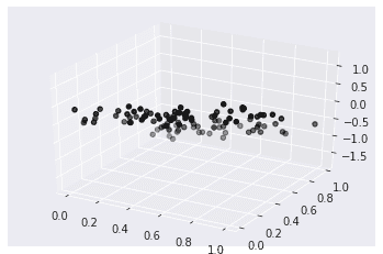
First, let’s prepare the dataset.

import numpy as np
import matplotlib.pyplot as plt
import seaborn as sns

sns.set_style("darkgrid")

n = 100
m = 2
X = np.random.rand(n,2)
y = X[:,0] - 2*X[:,1] + 0.5*np.random.rand(n)

fig = plt.figure()
ax = fig.add_subplot(111, projection='3d')
ax.scatter(X[:,0], X[:,1], y, color='k')
plt.show()

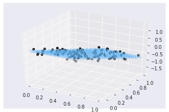
Next, call LinearRegression, fit the model, and plot the regression plane in 3D space.

from sklearn.linear_model import LinearRegression
from sklearn.metrics import r2_score

model = LinearRegression()
model.fit(X, y.reshape(-1, 1))

xx, yy = np.meshgrid(np.linspace(0, 1, 20), np.linspace(0, 1, 20))
model_viz = np.array([xx.flatten(), yy.flatten()]).T
predicted = model.predict(model_viz)

fig = plt.figure()
ax = fig.add_subplot(111, projection='3d')
ax.scatter(xx.flatten(), yy.flatten(), predicted, facecolor=(0,0,0,0), s=20, edgecolor='#70b3f0')
ax.scatter(X[:,0], X[:,1], y, color='k')
plt.show()

$R^2$ is also calculated in the same way.

r2_score(y, model.predict(X))
# >> 0.9640837457111405

References

[1] 倉田 博史, 星野 崇宏. “入門統計解析”（第9章）. 新世社. 2009.
[2] Multiple Linear Regression and Visualization in Python | Pythonic Excursions