The correlation coefficient is a familiar statistic, but there are several variations whose differences should be noted. This post recaps the definitions of these common measures.
The correlation coefficient is a familiar statistic that we see everywhere from news articles to scientific papers, but there are several variations whose differences should be noted. This post aims to recap the definitions of those common correlation coefficients, with the derivation of the equation and experiment regarding Spearman rank correlation coefficient.
Pearson Correlation Coefficient
For measuring the linear correlation between two sets of data, it is common to use Pearson product-moment correlation coefficient. Pearson correlation coefficient is the most well-known measure for correlation. When the term “correlation coefficient” is used without further information, it usually refers to this type of definition. Given paired data {(xi,yi)}i=1n, Pearson’s r is defined as:
where xˉ and yˉ are the sample means. The numerator is the covariance between xi and yi and the denominator is the product of their standard deviations.
The correlation coefficient ranges from −1 to 1. r=±1 is observed if and only if all the data points lie on a line (perfect correlation).
Spearman Rank Correlation Coefficient
When the data is ordinal variable, you should consider rank correlation. One of the common measures for rank correlation is Spearman rank correlation coefficient, which is simply the Pearson correlation coefficient between the two rank variables. For the n paired ranks {(ai,bi)}i=1n for the raw scores {(xi,yi)}i=1n, the Spearman’s ρ is defined as:
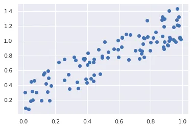
Here, I conducted a quick experiment to confirm that the Pearson’s r of the ranks is equivalent to Spearman’s ρ. I generated 100 pairs of random samples (x and y) and calculated several types of correlation coefficients.
import numpy as npimport matplotlib.pyplot as pltimport seaborn as snssns.set_style("darkgrid")n = 100x = np.random.rand(n)y = x + 0.5*np.random.rand(n)
Kendall rank correlation coefficient is another common type of rank correlation efficients. Among N pairs of indices {(i,j)}i<j, it considers the number of concordant pairsP, the number of discordant pairsQ, and ties Tx and Ty.
Given these quantities, Kendall’s τ (a) is defined as:
τa=NP−Q.
As well as Spearman’s ρ, Kendall’s τ (a) takes the value 1 if the order of the raw scores all match, and the value -1 if the order is completely reversed.
Kendall’s τ (b) cares about the case where ties are around.
τb=N−TxN−TyP−Q
Goodman and Kruskal’s Gamma
Simlarly, Goodman and Kruskal’s γ is defined as:
γ=P+QP−Q.
When there are no ties (i.e. Tx=Ty=0), Kendall’s τa and τb are equal to Goodman and Kruskal’s γ:
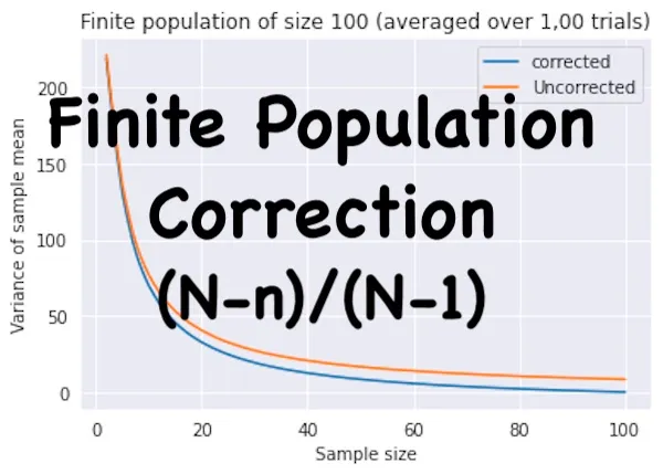
When you sample from a finite population without replacement, beware the finite population correction. The samples are not independent of each other.
2021-01-29 · 4 min read · EN
Shion Honda
Software engineer based in Rome since February 2026. I work on bringing AI agents into products, and I write about evaluation, context engineering, and the practical edges of LLM systems.