The Kaggle competition “HuBMAP + HPA - Hacking the Human Body”, which is about organ segmentation, ended on September 30. More than 1,000 teams joined the competition, and I came in 176th (top 15%).

What made it different from many other medical image competitions was its twist in how to split the dataset; the distributions of the train, public test, and private test sets were all different. For those who didn’t participate, this post describes the problem setting and summarizes the top solutions and my experience.

Problem Setting

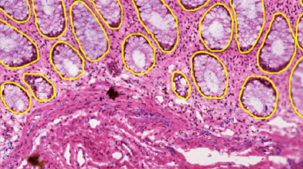
The task is to segment the organ region from a given tissue section image. The dataset includes five types of organs, and the organ type can be used as additional information along with pixel size, tissue thickness, and data source. There are two data sources: HuBMAP and HPA. They are drastically different from each other. Imaging conditions, staining protocols, and organ distribution are all different. You can get a sense of it from the figure below.

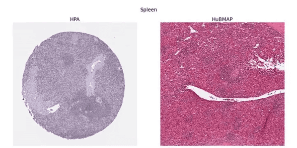
The twist is in how to split the dataset. The train set consists of HPA data only. The public test set is a mixture of HPA and HuBMAP. And the private test set consists of HuBMAP data only. The competition was a Code Competition, meaning that you have no access to the test data. So, here is the challenge: generalize to HuBMAP data given HPA data only.

The evaluation metric is Dice coefficient, which is defined as below:

where $X$ is the set of predicted pixels, $Y$ is the ground truth, and $|\cdot|$ computes the size of the operand.

For more detail, please refer to the official description.

Winners’ Solutions

The top five public solutions share several common features.

• Heavy augmentations helped models generalize to the HuBMAP data. Normalizing the pixel values was not enough at all. As far as I know, without heavy augmentations, nobody obtained good results on the HuBMAP data.
• UNet of large encoders was the de facto standard. Larger models performed better. Popular backbones were SegFormer, CoaT, and EfficientNet.
• Larger input images were also the key to better scores, which means “VRAM really matters” in this competition.
• Test time augmentations (TTA) could boost your score easily. Since they are tissue section images, you could apply flip augmentation 8 times (horizontal x vertical x mirror).
• External datasets & pseudo labels could also boost your score but required more effort.

1st Place

Opusen took first place by looking at the labels carefully. The key to the victory was the hand-labeling of lung images. They noticed that the noisy labels in lung images lead to unstable results, which motivated them to re-label those images manually.

I’d also like to mention their normalization technique. They wanted to train SegFormers (MiT) at the resolution of 1024x1024, but the VRAM of Google Colaboratory was not enough. They solved this problem by using group normalization with the batch size of 1 instead of batch normalization, which somehow improved the score at the same time.

2nd Place

Victor Durnov used various large models:

• EfficientNet B7
• EfficientNetV2 L
• ConvNeXt L
• CoaT-Lite Medium

3rd Place

Human Torus Team’s approach is similar to others, but I’d like to highlight two points here. First, they used CutMix for data augmentation. Second, at inference time, they used images in full scale. When the image was too large to fit in the memory, they split it into small tiles and concatenated the outputs.

4th Place

Rock didn’t use external data or pseudo labels. Instead, they utilized stain (color) normalization.

7th Place

Q_takka won a gold medal using Kaggle Notebook only. Due to the memory limit, they used slightly smaller models like EfficientNet B5 and input images of 800x800 resolution. To overcome these constraints, they carried out inference in two ways and averaged the outputs: (1) inference on the whole image and (2) concatenation of the prediction of tiled images.

My Experience

I had trouble in the computing environment (which was resolved at the very end of the competition), so I couldn’t increase the model size and image size as I wanted. The final solution looks like this:

• 😀 Heavy augmentations
• 😐 UNet of medium encoders
• 😐 Medium-sized input images
• 😀 TTA
• 😰 No external datasets or pseudo labels

Finally, I’d like to add some comments on the thresholding algorithm. The evaluation metric, the Dice coefficient, is very sensitive to the threshold you choose. This means that the threshold must be adjusted each time you want to evaluate the model. To make matters worse, the optimal thresholds are different for the train set (HPA) and the test set (HuBMAP). It’s almost impossible to tune the threshold using the leaderboard score! To address this issue, I used an automatic thresholding algorithm called Otsu’s binarization. Otsu’s method is essentially a discriminant analysis for binarizing images. You can use it easily with OpenCV. In my experiments, Otsu’s method performed comparable to manual tuning and better than adaptive thresholding algorithms.